
Google Sheets offers a variety of powerful functions to streamline your data management and analysis tasks. One such function is HLOOKUP, which stands for Horizontal Lookup. This guide will walk you through how to use the HLOOKUP function in Google Sheets, complete with examples and practical applications. By the end of this article, you will understand how to implement HLOOKUP to efficiently retrieve data from your spreadsheets.
What is HLOOKUP?
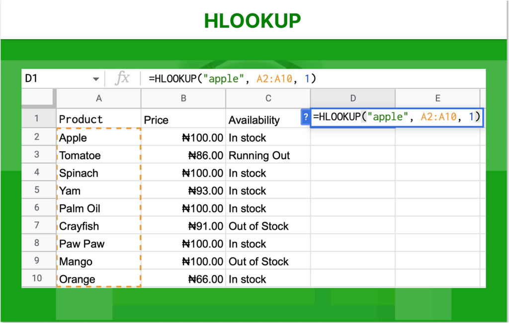
HLOOKUP (Horizontal Lookup) is a function in Google Sheets used to search for a specific value in the first row of a table or range and return a value in the same column from a specified row. It’s particularly useful when dealing with data organized horizontally across the top row of your sheet.
Syntax of HLOOKUP
The syntax for the HLOOKUP function is:
scssCopy codeHLOOKUP(search_key, range, index, [is_sorted])
- search_key: The value you want to search for in the first row of the range.
- range: The table or range where you want to search and retrieve the data.
- index: The row number in the range from which to return the value.
- is_sorted: An optional argument that indicates whether the first row of the range is sorted. By default, it is TRUE. If set to FALSE, an exact match is required.
How to Use HLOOKUP in Google Sheets
Let’s break down the steps to use HLOOKUP effectively with a few examples.
Example 1: Basic HLOOKUP
Suppose you have the following data in your Google Sheet:
| A | B | C | D | |
|---|---|---|---|---|
| 1 | Product ID | P001 | P002 | P003 |
| 2 | Price | 20 | 30 | 25 |
| 3 | Stock | 50 | 40 | 60 |
You want to find the price of Product ID “P002”.
- Identify the search_key: In this case, it is “P002”.
- Define the range: The range to search within is A1.
- Specify the index: Since prices are in the second row, the index is 2.
- Set is_sorted: If your data is not sorted, set this to FALSE.
The HLOOKUP formula will be:
phpCopy code=HLOOKUP("P002", A1:D3, 2, FALSE)
This will return 30, the price of Product ID “P002”.
Example 2: HLOOKUP with Dynamic References
Suppose you have a dropdown menu to select a product ID and you want the price to update automatically based on the selected ID.
- Create a dropdown: In cell F1, create a dropdown list with product IDs.
- Use HLOOKUP with a cell reference: Reference the cell with the dropdown in your HLOOKUP formula.
Assuming the dropdown is in cell F1, the formula becomes:
phpCopy code=HLOOKUP(F1, A1:D3, 2, FALSE)
Now, when you select a different product ID from the dropdown, the price will update accordingly.
Example 3: HLOOKUP with Nested Functions
You can use HLOOKUP in combination with other functions to perform more complex operations. For instance, you might want to calculate the total stock value for a specific product.
Using the same data, if you want to find the total stock value of “P001”, you can use HLOOKUP and multiplication:
phpCopy code=HLOOKUP("P001", A1:D3, 2, FALSE) * HLOOKUP("P001", A1:D3, 3, FALSE)
This formula retrieves the price and stock for “P001” and multiplies them to give the total stock value.
Practical Applications of HLOOKUP
HLOOKUP is versatile and can be used in various scenarios to enhance your data analysis capabilities. Here are a few practical applications:
Financial Analysis
In financial spreadsheets, you can use HLOOKUP to pull specific financial metrics from a table based on a given time period or criteria. For instance, you could retrieve quarterly sales figures or expense data for specific months.
Inventory Management
For businesses managing inventory, HLOOKUP can help retrieve stock levels, pricing information, and reorder points for various products, streamlining inventory audits and reordering processes.
Educational Tools
Teachers and administrators can use HLOOKUP to quickly access student grades, attendance records, and other important metrics based on student IDs or names.
Project Management
Project managers can use HLOOKUP to fetch data on project timelines, resource allocation, and task status from a comprehensive project tracking sheet.
Tips for Using HLOOKUP Effectively
1. Ensure Data Consistency
Make sure the first row of your range (where HLOOKUP searches) contains unique and consistent values. This ensures accurate and reliable results.
2. Use Absolute References
When copying formulas across cells, use absolute references (e.g., $A$1:$D$3) to keep the range fixed.
3. Combine with Other Functions
Combine HLOOKUP with other Google Sheets functions like IF, SUM, or INDEX for more complex data manipulation and analysis.
4. Validate Inputs
If using dynamic inputs like dropdowns, validate the inputs to ensure they match the values in your data range to avoid errors.
5. Keep Data Sorted
Although HLOOKUP can work with unsorted data by setting is_sorted to FALSE, keeping your data sorted can improve performance and make your sheet easier to navigate.
Conclusion
HLOOKUP in Google Sheets is a powerful function for retrieving data based on specific criteria from horizontally organized tables. By following the steps and examples provided in this guide, you can harness the full potential of HLOOKUP to enhance your data management and analysis tasks. Whether you are managing financial data, inventory, educational records, or project timelines, HLOOKUP offers a versatile solution for quick and accurate data retrieval.
For more insights on enhancing your data analysis skills and staying updated with the latest financial news, check out our article on FintechZoom News.

Jason Bennett is a tech enthusiast and software engineer with a passion for the latest gadgets and technological advancements. With a decade of experience in the tech industry, Jason offers in-depth reviews, analyses, and tips on the newest devices and software. His expert knowledge and keen eye for detail make him a trusted voice in the world of technology.


